BxD Primer Series: Stable Diffusion Models

Stable diffusion models are able to progressively refine a simple distribution, to generate visually compelling data that closely resemble real-world observations.

Jun 01, 2023

Hey there 👋

Welcome to BxD Primer Series where we are covering topics such as Machine learning models, Neural Nets, GPT, Ensemble models, Hyper-automation in ‘one-post-one-topic’ format. Today’s post is on Stable Diffusion Models. Let’s get started:

Introduction to Diffusion Process and Stable Process:

Diffusion is a concept in physics that describes the behavior of particles as they spread and mix due to random motion. It is a process to model movement of particles from high concentration to of low concentration areas, resulting in equal concentration gradient over time.

Main properties of diffusion:

Diffusion occurs due to random motion of particles. Individual particles move independently and randomly, continuously changing its direction and velocity.
Diffusion takes place when there is difference in concentration of particles between two regions. Particles move from higher concentration to lower concentration areas.
Diffusion coefficient, denoted as D, measures how quickly particles spread out and mix. It depends on the nature of particles and the medium in which they are diffusing.
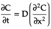
Fick's laws provide a mathematical description of diffusion.
- First law: Rate of diffusion is proportional to concentration gradient.
  J = -D(dC/dx)
  Where,
  - J is the diffusion flux (amount of particles crossing a unit area per unit time)
  - C is the concentration
  - x is the position
  - dC/dx is the concentration gradient
- Second law: Change in concentration over time is proportional to second derivative of concentration w.r.t. position.

✪ Diffusion processes have properties of continuity, Markovian behavior, and a tendency to spread out and mix due to random motion. They are used to model phenomena of molecular transport, heat conduction, stock price movements, and more.

In stable diffusion models, the ideas of diffusion process are combined with stable processes, also known as Lévy processes.

✪ Stable processes have properties of heavy-tailed distributions and absence of finite variance. They are characterized by stable distributions, with parameters such as stability index, scale parameter, skewness parameter, and location parameter.

Note: There are many new terminology introduced here, we will keep explaining them in detail as this post progresses.

Terminology Explanation:

Terminology around stable diffusion models:

Definition: Stable diffusion is a stochastic process (and not deterministic) with following properties:
- Stationarity: Meaning that its statistical properties do not change over time.
- Increments (individual steps or iterations in diffusion process) are independent and identically distributed.
- Distribution of increments are stable, characterized by heavy tails and infinite variance.
Stable distributions: A generalization of Gaussian (normal) distribution, characterized by four parameters:
- Stability index α ∈ (0, 2]: It determines the shape of distribution. When α = 2, the distribution reduces to a Gaussian distribution.
  α > 2 correspond to finite variance and α < 2 correspond to infinite variance.
- Scale parameter σ > 0: It scales the distribution and controls dispersion.
- Skewness parameter β ∈ [-1, 1]: It introduces skewness to distribution.
- Location parameter μ: It shifts the distribution along x-axis.
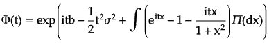
Stable diffusion models can be represented using Levy-Khintchine formula, which is a relation between characteristic function of process and its parameters:
Where,
- i is the imaginary unit, defined as i^2= −1
- t is the parameter space of characteristic function. It can be thought as the time variable.
- x is the variable set representing the argument of Levy measure.
- b is the drift parameter, which represents rate of change of process over time.
- σ^2 is the diffusion parameter, which quantify the variance or spread of process over time.
- Π(dx) is the Levy measure, which characterize jump behavior of Levy process. It is a measure defined on the real line that describes the distribution of the jumps or discontinuities in the process.
Levy measure is the intensity of jumps (discrete steps during diffusion process where the distribution is transformed) in the process.

Note: Increment independence means that:

For a stable diffusion process X(t) with time parameter t, the increments ΔX(t) = X(t + Δt) − X(t) for different time intervals Δt are independent random variables.
In other words, the behavior of process in one interval does not depend on or influence the behavior in other intervals.

The What:

Stable diffusion models combine the properties of stable processes and diffusion processes. Stable processes are characterized by heavy-tailed distributions and independent increments, diffusion processes describe the random motion of particles or variables over time.

Properties of stable diffusion models:

Heavy-tailed distributions: Meaning that they can model processes with a high likelihood of extreme events or outliers, such as financial asset returns, where extreme events occur more frequently than would be expected under a normal distribution.
Heavy-tailed nature also ensures that the model can handle extreme events or outliers without destabilizing the training process.
Diffusive behavior: Heavy-tailed distribution models extreme events, while diffusive behavior captures the overall spread or mix of data into process. It enables the model to consider information from distant regions of data and still generate globally consistent samples.
Infinite variance implies that the model can represent extreme fluctuations. This character arises from heavy-tailed nature of stable distributions.
Captures multi-modal distributions: Real-world datasets exhibit multiple modes or clusters, for distinct patterns or groups within data. Stable diffusion models can effectively generate samples from multi-modal data, resulting in diverse and varied outputs.

Note: Heavy-tailed nature of stable distribution is quantified by the stability index (α). Values of α between 0 and 2 indicate heavy-tailed behavior, with lower values indicating heavier tails.

The How:

General steps to build stable diffusion models:

Start with a base distribution, p_0(x), where x is the input data or latent space variables. It is typically a standard Gaussian distribution.
Define the diffusion process: Diffusion process aims to transform base distribution p_0(x) into a more complex distribution p_T(x).
This is done by applying a series of invertible transformations f_t over T steps.
Each step involves a transformation f_t and an associated noise term u_t.
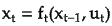
Where,
- x_t is the output at step t
- x_{t−1} is the input from previous step
- u_t is the noise term.
Define the transformation function: Transformation function f_t is typically implemented using neural networks or other suitable architectures.
Specify the noise term: Noise term u_t is typically modeled as independent and identically distributed Gaussian noise with zero mean and a variance that changes (usually decreases) over diffusion steps.
Learn the parameters: Train the model to learn parameters of transformation function f_t and optimize them to minimize a suitable loss function, such as maximum likelihood estimation or variational inference.
Training process involves updating parameters using gradient-based optimization algorithms such as stochastic gradient descent (SGD) or Adam.
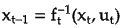
Sampling from the model: Once model is trained, you can generate samples by iteratively applying learned transformation steps to base distribution. Starting with a sample x_0 from base distribution, apply the inverse transformations in reverse order:
where f_t^{−1} is inverse transformation function.
Evaluation and refinement: Evaluate the performance of the model by assessing metrics such as sample quality, diversity, and fidelity to the target distribution. If necessary, iterate and refine the model by adjusting hyperparameters, architecture choices, or training procedures to improve its performance.

Parameter in Stable diffusion model:

Several parameters and hyper-parameters define the characteristics of stable diffusion model:

Parameters for stable distributions:
- Stability index (α) determines the tail heaviness of stable distribution.
- Scale parameter (β) controls the spread of stable distribution.
- Skewness parameter (γ) captures the asymmetry of stable distribution.
- Location parameter (μ) represents the center or location of stable distribution.
Parameters for diffusion process:
- Drift coefficient (μ) determines the mean behavior of diffusion process.
- Diffusion coefficient (σ) controls the volatility or randomness of diffusion process.
Time step (Δt) defines the interval at which diffusion process is discretized. It determines the granularity of continuous diffusion process.
Initial value (X0) is the starting point of diffusion process.
Time horizon (T) specifies the duration of diffusion process (period over which the model generates samples).
Number of time steps (N) refers to total number of iterations in diffusion process. It is related to time horizon and time step size and affects the resolution and accuracy of output.
Noise distribution determines the type of distribution from which the random fluctuations are drawn, such as Gaussian, Cauchy, or Levy.
Network architecture: In most modern stable diffusion models, neural network architecture is used to parameterize drift and diffusion coefficients. Network parameters - number of layers, hidden units, activation functions, etc., affects expressive power and capacity of model.
Loss function defines the objective that model aims to minimize during learning process and can be tailored based on specific task at hand.

The Why:

Reasons for using Stable Diffusion Models:

Can accurately represent and generate samples from distributions with extreme events and outliers, called heavy-tailed characteristics, which are often observed in real-world data
Can effectively handle and model data points that deviate significantly from bulk of the distribution. This encourages diversity in generative stable diffusion models.
Can capture long-range dependence or correlations and memory effects in data.
Allows for modeling of processes that evolve continuously over time, useful for high-frequency or time-sensitive data.
Can effectively model nonlinear dynamics, capturing complex relationships and interactions in data.

The Why Not:

Reasons for not using Stable Diffusion Models:

There are multiple hyper-parameters in model which need to be tuned to get a good fit on data and task at hand.
Lack closed-form analytical solutions, which makes user to rely on approximation techniques for inference.
Require a substantial amount of data to accurately estimate model parameters and capture underlying dynamics.
Lack of standardized implementations or libraries compared to more established modeling techniques.
With their complex distributions and diffusive behavior, these models are less interpretable compared to simpler models like Gaussian-based approaches.
Stable diffusion models are capable of capturing complex data distributions, but this flexibility can also lead to overfitting when the dataset is limited or noisy.